Bezier Curve with deCasteljau Algorithm
Introduction
The deCasteljau’s algorithm introduces a way to create Bezier curves through the evaluation of Bernstein polynomials. A Bezier curve is a parametric polynomial curve that uses polynomials for its coordinates functions [1]. Consequently, an nth-degree Bezier curve is defined by
\[\textbf{C}(u) = \sum^n_{i=0}B_{i,n}(u)\textbf{P}_{i} \qquad 0 \leq u \leq 1.\]The set $\{\textbf{P}\}$ are called control points, and the $B_{i,n}(u)$ are Bernstein polynomials. The control points are the geometric coefficients of the Bezier curve and the Bernstein polynomials are basis functions. Therefore, the curve $\textbf{C(u)}$ can be expressed as a linear combination of the control points and Bernstein polynomials. Consequently, the deCasteljau’s algorithm recursively iterates over the control points to produce a numerical stable Bezier curve.
Bernstein polynomials gives a formulation for building Bezier curves of any degree. The Bernstein polynomials $B_{i,n}$ are defined as
\begin{equation} B_{i,n}(u) = \frac{n!}{i!(n-i)!}u^i(1-u)^{n-i} \qquad 0 \leq u \leq 1. \end{equation}
However, the deCasteljau’s algorithm avoids the direct calculation of factorials. Instead, it exploits the Bernstein polynomials property where $B_{0,n}(0) = B_{n,n}(1) = 1$, and it produces a point on the curve by recursion. In addition, the partition of unity property $ \sum^n_{i=0}B_{i,n}(u) = 1 \quad \forall u \in [0,1]$ ensures the interpolation between the control points.
Example
For this example, let’s create a quadratic Bezier curve. A quadratic Bezier curve represents the case for $n = 2$ in the definition above. Using the property $B_{0,n}(0) = B_{n,n}(1) = 1$ the Bernstein polynomials take the following form
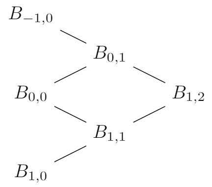
\[B_{0,1}(u) = (1-u)B_{0,0}(u) + uB_{-1,0}(u) = 1 - u \\ B_{0,1}(u) = (1-u)B_{1,0}(u) + uB_{0,0}(u) = u \\ B_{0,1}(u) = (1-u)B_{0,1}(u) + uB_{-1,0}(u) = (1 - u)^2 \\ B_{0,1}(u) = (1-u)B_{0,0}(u) + uB_{-1,0}(u) = (1 - u)u + u(1-u) = 2u(1 - u) \\ B_{0,1}(u) = (1-u)B_{2,1}(u) + uB_{1,1}(u) = 1 - u\]This a direct result of using the recursive property of the basis functions. In addition, from the figure below shows the set of recursive dependency for the of $B_{1,2}$
Then the curve formed by control points $\{ \textbf{P}_0, \textbf{P}_1, \textbf{P}_2 \}$ is
\[\textbf{C(u)} = B_{0,2}P_0 + B_{1,2}P_1 + B_{2,2}P_2 = (1-u)^2P_0 + 2u(1-u)P_1 + u^2P_2\]Implementation
OpenGL Setup
For drawing the curve I will be using modern OpenGL; the setup will use vertex and fragment shaders. I followed this tutorial for the basic setup. In addition, the data will be computed with the CPU, then with pass this data to OpenGL drawing functions for the GPU to draw it.
For the implementation, the algorithm will be encapsulated in a class. A curve class will contain the algorithm, so we could reuse it and implement other algorithms for curve creation.
deCasteljau Algorithm
We would like to display a 2D curve, therefore, having a struct with an x and y coordinates will come very handy. By defining a struct Point with two coordinates we can create a vector of points, which can then be used for the algorithm. Thus, it just makes sense to create a vector that holds a collection of 2D points for the control points. In addition, we will use the same data structure to copy the control points in a temporary vector of points, which will produce the points for the Bezier curve.
#ifndef CURVE_H
#define CURVE_H

#include <vector>
struct Point {
    float x;
    float y;
};

class Curve{
public:
    Curve() = default;
    const std::vector<float>& deCasteljau(std::vector<float>& ctrl_pts);
private:
    void deCasteljau_Subroutine(float u);
    void Vector_To_Points(std::vector<float>& ctrl_pts);
    std::vector<float> m_curve;
    std::vector<Point> m_ctrl_pts;
};
#endif
static const float m_res = 0.001f;

const std::vector<float>& Curve::deCasteljau(std::vector<float>& ctrl_pts){
    Vector_To_Points(ctrl_pts);

    if(!m_curve.empty()) m_curve.clear();

    for(float u = 0.0f; u < 1.0f; u += m_res){
        deCasteljau_Subroutine(u);
    }

    return m_curve;
}

void Curve::deCasteljau_Subroutine(float u){
    std::vector<Point> tmp_ctrl_pts(m_ctrl_pts);
    for(int i = 1; i < tmp_ctrl_pts.size(); i++){
        for(int j = 0; j < tmp_ctrl_pts.size() - i; j++){
            tmp_ctrl_pts[j].x = (1.0f - u) * tmp_ctrl_pts[j].x + u * (tmp_ctrl_pts[j + 1].x);
            tmp_ctrl_pts[j].y = (1.0f - u) * tmp_ctrl_pts[j].y + u * (tmp_ctrl_pts[j + 1].y);
        }
    }

    m_curve.emplace_back(tmp_ctrl_pts[0].x);
    m_curve.emplace_back(tmp_ctrl_pts[0].y);
    m_curve.emplace_back(0.0f);             // the curve lives in the xy plane (x, y, z = 0)
}
The code for the project can be found here.

